The Semantic Revolution: Lexical vs Vector Search
BM25 matches literal keywords. If a user searches for "canine wellness clinic", BM25 fails to match a document titled "dog veterinarian hospital" because zero vocabulary terms overlap. Vector Search maps text into dense high-dimensional semantic vector spaces (e.g. 1536-dimensional embeddings generated by neural models) where semantically similar concepts cluster together.
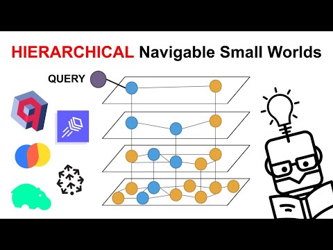
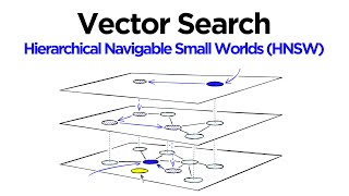
HNSW (Hierarchical Navigable Small World) Graph Architecture
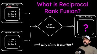
Under the Hood: Hybrid Search Fusion (RRF)
Vector search excels at broad semantic concept matching but frequently fails on exact keyword identifiers (e.g. part numbers like "GTX-4090-TI" or specific product codes). The industry gold standard is Hybrid Search, combining lexical BM25 and dense vector search using Reciprocal Rank Fusion (RRF):
RRF_Score(d) = sum_{m in Models} ( 1 / (60 + Rank_m(d)) )RRF normalizes disparate scoring scales into rank positions, ensuring that documents ranking well across both keyword matching and semantic embedding models float to the top.
Worked example: memory for 100 million vectors
| Component | Calculation | Size |
|---|---|---|
| Raw float32 vectors, 768 dimensions | 100,000,000 x 768 x 4 bytes | about 307 GB |
| HNSW base-layer links, M = 16 | 2M = 32 neighbours x 4 bytes x 100,000,000 | about 12.8 GB, upper layers add a little more |
| Product-quantised codes, 96 bytes per vector | 100,000,000 x 96 bytes | about 9.6 GB |
| int8 scalar quantisation | 100,000,000 x 768 x 1 byte | about 77 GB |
This is why large deployments shard vectors across many nodes and use quantised vectors for the graph search, then re-score the top few hundred candidates with full-precision vectors.
Worked example: reciprocal rank fusion
RRF score = sum over rankers of 1 divided by (60 + rank).
| Doc | BM25 rank | Vector rank | RRF score |
|---|---|---|---|
| X | 1 | 20 | 1/61 + 1/80 = 0.0289 |
| Y | 5 | 3 | 1/65 + 1/63 = 0.0313 |
| Z | 2 | not returned | 1/62 = 0.0161 |
Y, which both systems like, wins over X, which only BM25 loves. The constant 60 comes from the original RRF paper (Cormack, Clarke and Buettcher, 2009) and dampens the advantage of a single first-place rank.
ANN index trade-offs
| Index | Speed and recall | Memory | Updates |
|---|---|---|---|
| Flat, brute force | Exact, slow at scale | Vectors only | Trivial |
| HNSW | Excellent recall at low latency | Vectors plus graph, highest | Inserts fine; deletes are usually tombstoned |
| IVF with PQ | Good, tunable via nprobe | Very compact | Needs training; periodic retraining |
| DiskANN-style graphs | Good, SSD-resident | Small RAM footprint | More complex |
Filtering pitfall: applying a restrictive filter such as tenant or in-stock after ANN search can leave too few results; engines such as Elasticsearch, OpenSearch, Vespa and Weaviate implement filtered HNSW traversal or fall back to exact search when the filter is very selective.
Tuning knobs that matter
For HNSW, M controls graph degree (memory and recall), ef_construction controls build quality, and ef_search controls the query-time candidate list. Raising ef_search from 40 to 200 commonly lifts recall at 10 from around 0.9 into the high 0.9s at a few times the latency. Measure recall against exact brute-force results on a sample of real queries, not synthetic ones.