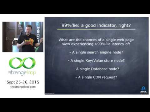

Architecting Streaming Percentiles
To provide real-time SLA dashboards, a system must process millions of latency metrics and output p90, p95, and p99 metrics instantaneously. This requires combining stream processing with sketch data structures.
The Pipeline
Applications emit raw latency events to a message broker (Kafka). A stream processing framework (Apache Flink) reads these events in time windows (e.g., 10-second tumbling windows). Inside the Flink operators, a t-digest or HDRHistogram sketch is updated in memory. At the end of the 10 seconds, the sketch is emitted to a Time-Series Database (TSDB).
Query Time Rollups
When a user opens an SLA dashboard and requests the p99 latency for the last 24 hours, the TSDB retrieves the thousands of stored 10-second sketches and merges them together on the fly. Merging thousands of sketches at every query can still be expensive, so retain hierarchical rollups with compatible parameters and contribution IDs. Validate approximation error against exact samples, and define whether late windows replace or add to a prior contribution.
Worked example: why rollups are needed
A service has 50 hosts and 20 endpoints, so 1,000 series. Sketches are emitted every 10 seconds.
| Query | Sketches merged without rollups | With 1-minute and 1-hour rollups |
|---|---|---|
| p99 last 5 minutes, one endpoint across all hosts | 30 buckets x 50 hosts = 1,500 | 5 x 50 = 250, or 5 if hosts are pre-merged |
| p99 last 24 hours, whole service | 8,640 buckets x 1,000 series = 8.64 million | 24 hourly service-level sketches |
At a few KB per sketch, 8.64 million sketches is tens of GB read per query, which is unusable. With rollups it is under a megabyte. Rollups must use the same sketch parameters so that merges remain valid, and must record which inputs were included so that late windows replace their contribution rather than being counted twice.
Pipeline
Client-side vs server-side aggregation
| Where the sketch is built | Pros | Cons |
|---|---|---|
| In the application, as HdrHistogram or Prometheus buckets | No per-request events on the wire; cheap | Fixed configuration at instrumentation time |
| In the stream processor from raw events | Can re-slice by any dimension; replayable | Ships every event; higher cost |
| In the database at query time from raw rows | Maximum flexibility | Slowest; scans raw data |
SLO alerting tip: for "99 percent of requests under 300 ms" it is often simpler and exact to count requests above and below 300 ms per bucket, two additive counters, rather than estimating the p99 and comparing it. Google's SRE guidance on SLOs uses exactly this good-events over total-events formulation.
Coordinated omission in one example
A load tester sends one request every 10 ms. The server stalls for 2 seconds. A naive tester that waits for each response records one 2-second sample and then continues, so the percentile report shows one slow request out of thousands. In reality about 200 requests (the ones that should have been sent during the stall) would have waited up to 2 seconds. HdrHistogram's recordValueWithExpectedInterval corrects for this; alternatively, use an open-loop load generator that sends on schedule regardless of responses.