Comparing Geospatial Grid Systems
When building large-scale spatial applications, choosing the right grid system is critical. Geohash, Google's S2, and Uber's H3 are the three most prominent grid systems, each with distinct characteristics and trade-offs.
Geohash (Rectangles)
Geohash divides the world into rectangles. Its main advantage is simplicity and native support in many databases. However, because the Earth is spherical, the actual physical area of Geohash rectangles varies significantly depending on the latitude. A Geohash near the equator covers much more area than one near the poles, making radius calculations inconsistent.
Google S2 (Quadrilaterals)
Google developed the S2 geometry library to solve the distortion problem. It maps the sphere to a cube and then recursively subdivides each face as a quadtree of quadrilateral cells, numbering those cells along a Hilbert curve so nearby cells usually get nearby IDs. S2 provides excellent precision and mathematical guarantees about cell sizes. It is widely used in systems like MongoDB and Foursquare.
Uber H3 (Hexagons)
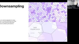
H3 indexes the sphere with mostly hexagonal cells plus required pentagons, across a hierarchy of resolutions. Neighbor traversal is convenient for aggregation and approximate coverings, but projection distortion means real-world cell areas and center distances are not identical everywhere. Radius and boundary decisions still require exact geometry or distance checks after candidate generation.
Summary of Trade-offs
| System | Shape | Best Use Case |
|---|---|---|
| Geohash | Rectangle | Simple string-based indexing, fast prototyping |
| S2 | Quadrilateral | General-purpose mapping, minimal distortion |
| H3 | Hexagon | Ride-sharing, continuous neighbor traversal |
Worked example: picking a resolution
Surge pricing wants zones of roughly neighbourhood size.
- H3 resolution 7 hexagons average about 5.2 square km, resolution 8 about 0.74 square km, resolution 9 about 0.11 square km. Each step divides area by about 7 (aperture 7). Resolution 8 gives about 1,600 cells over a 1,200 square km city.
- S2 has 31 levels (0 to 30). Level 13 cells average about 1.3 square km and each level divides area by exactly 4; a level 30 cell is under a square centimetre. Cell IDs are 64-bit integers ordered along a Hilbert curve, so a region covering is a small set of integer ranges.
- Geohash precision 6 gives 1.2 km by 0.6 km cells at the equator, but only about 0.6 km wide at 60 degrees latitude, so zone areas vary with latitude.
Comparison
| Property | Geohash | S2 | H3 |
|---|---|---|---|
| Cell shape | Lat/lon rectangle | Spherical quadrilateral | Hexagon (plus 12 pentagons) |
| Hierarchy | Exact nesting, 32 children | Exact nesting, 4 children | Approximate nesting, 7 children |
| ID ordering | Z-order curve (base32 string or integer) | Hilbert curve (64-bit integer) | Hierarchical 64-bit index, not a locality-preserving range |
| Area distortion | Large, grows toward poles | Small (roughly 2x across the globe) | Small (roughly 2x across the globe) |
| Neighbours | 8, at two distances | 8 (edge plus vertex) | 6, all at one distance |
| Best at | Simple prefix queries in any database | Region coverings and range scans | Aggregation, smoothing, movement between cells |
| Known users | Redis GEO, Elasticsearch grids | Google, MongoDB 2dsphere, Tinder geosharding | Uber marketplace and surge, many analytics tools |
Common patterns
- Coverings: S2's RegionCoverer turns a circle or polygon into a bounded number of cells at mixed levels (for example max 8 cells), trading over-coverage for fewer lookups.
- k-rings: H3's gridDisk(cell, k) returns all cells within k steps, which approximates a radius and is ideal for "demand near this driver".
- Sharding: assign coarse cells (S2 level 5 or H3 resolution 2 or 3) to shards; hot cities may need to be split further.