
The Foundations of Lexical Relevance
How does a search engine decide whether Document A is more relevant to a query than Document B? The foundational mathematical model of information retrieval is TF-IDF (Term Frequency - Inverse Document Frequency).
The Two Core Components of TF-IDF
Under the Hood: The Mathematical Formulas
1. Term Frequency (TF)
Measures how frequently term t occurs in document d. The simplest form is raw count freq(t, d), but modern systems apply logarithmic damping to prevent documents with 100 mentions of a word from dominating documents with 10 mentions:
TF(t, d) = 1 + ln(freq(t, d)) (for freq > 0)2. Inverse Document Frequency (IDF)
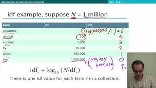
Common words (e.g. "the", "system") appear in almost every document and provide zero discriminatory power. Rare words (e.g. "Paxos", "Bloom") carry high information entropy. Given total documents N and document frequency DF(t):
IDF(t) = ln(1 + (N / DF(t)))3. The Vector Space Model (Cosine Similarity)
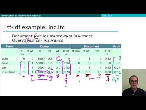
Documents and queries are represented as high-dimensional vectors in term space. The relevance score is computed as the cosine of the angle between query vector q and document vector d:
Cosine_Similarity(q, d) = (q . d) / (||q|| * ||d||)Worked example: why the log matters
Corpus: N = 1,000,000 documents. Query: raft system.
| Term | DF | IDF = ln(1 + N/DF) |
|---|---|---|
| raft | 1,000 | ln(1001) = 6.91 |
| system | 400,000 | ln(3.5) = 1.25 |
Document A mentions raft 3 times and system 10 times. Document B mentions raft once and system 30 times.
| Scoring | Doc A | Doc B | Winner |
|---|---|---|---|
| Raw TF x IDF | 3 x 6.91 + 10 x 1.25 = 33.3 | 1 x 6.91 + 30 x 1.25 = 44.5 | B |
| Log TF x IDF, TF = 1 + ln f | 2.10 x 6.91 + 3.30 x 1.25 = 18.6 | 1.00 x 6.91 + 4.40 x 1.25 = 12.4 | A |
With raw counts, B wins by repeating a near-useless word. With log damping, A wins because it talks more about the rare, discriminating term. This is the core lesson of TF-IDF.
Cosine normalisation in one line
Dividing by vector length means a 10,000-word document is not rewarded simply for containing more terms. In practice engines precompute each document's norm at index time so query-time cost stays proportional to the query's postings.
TF variants compared
| TF form | Behaviour | Used in |
|---|---|---|
| Raw count | Linear, easily gamed by repetition | Teaching examples |
| 1 + ln f | Grows slowly but without bound | Classic SMART lnc.ltc schemes |
| sqrt f | Sub-linear | Lucene ClassicSimilarity, the pre-BM25 default |
| BM25 saturation | Bounded, tunable, length-aware | Default in Lucene 6 and later, Elasticsearch 5 and later |
Failure modes: IDF computed per shard can differ across shards when documents are unevenly distributed, which is why Elasticsearch offers a dfs_query_then_fetch mode that gathers global term statistics first; tiny corpora produce noisy IDF values.
Interview framing
If asked "how would you rank documents for a keyword query?", start with TF-IDF to show you understand the two forces, local frequency and global rarity, then say production engines use BM25 because it bounds repetition and normalises length with tunable parameters, and finally mention a learned re-ranker on top for non-text signals such as popularity and freshness. That three-step answer covers the evolution from 1970s vector space models to modern two-stage ranking.