

Search Service Architecture Overview
A production search service (like Elasticsearch, Solr, or internal enterprise search) consists of two decoupled subsystems: the Write/Indexing Pipeline and the Read/Query & Ranking Engine. The goal is to ingest documents, extract terms, compute relevance, and serve full-text queries in under 50 milliseconds across billions of documents.
Indexing & Query Flow
Inverted Index & Posting Lists
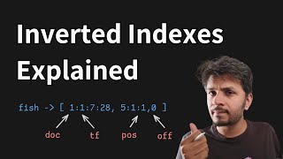
Rather than scanning records sequentially, search engines build an inverted index mapping each tokenized word to a sorted list of document IDs (called a posting list):
"distributed" -> [Doc1, Doc4, Doc12, Doc98]
"systems"     -> [Doc2, Doc4, Doc15, Doc98]
Boolean conjunction queries (distributed AND systems) intersect sorted posting lists in O(N + M) time using skip lists or bitset operations.
Relevance Scoring: BM25
Relevance ranking evaluates how well a document matches a query based on Best Matching 25 (BM25), balancing:
- Term Frequency (TF): How often the term appears in the document (with diminishing returns).
- Inverse Document Frequency (IDF): How rare the term is across the entire corpus (common words like "the" receive low weight).
- Field-Length Normalization: Term frequency is normalized by document length relative to the average (BM25's b parameter), so the same match counts for more in a short document than in a long one.
Worked example: BM25 inverse document frequency
The corpus has N = 1,000,000 documents. Lucene's BM25 IDF is ln(1 + (N - n + 0.5) / (n + 0.5)), where n is the number of documents containing the term.
- "kafka" appears in n = 1,000 documents:
ln(1 + 999000.5 / 1000.5), which is aboutln(1000), about 6.9. - "system" appears in n = 400,000 documents:
ln(1 + 600000.5 / 400000.5), which isln(2.5), about 0.92. - "the" appears in n = 950,000 documents: about
ln(1.053), about 0.05, which is effectively noise.
The term-frequency part saturates. With Lucene's defaults k1 = 1.2 and b = 0.75, a term appearing 10 times scores only about 2 times as much as appearing once in a document of average length. Longer-than-average documents are damped by the b parameter. So a match on "kafka" is worth about 7 times a match on "system", no matter how often "system" repeats.
How to partition the index
| Strategy | Query path | Write path | Used by |
|---|---|---|---|
| Document-partitioned (each shard indexes a subset of documents) | Scatter to every shard, gather top K from each, merge | Each document goes to one shard | Elasticsearch, Solr, most production systems |
| Term-partitioned (each shard owns some terms) | Only the shards holding the query's terms | One document updates many shards | Rare; research systems and some early web search engines |
| Tiered (a small fresh index plus a large base index) | Query both and merge | New documents go to the fresh tier | Web search engines, Twitter's Earlybird real-time index |
Latency budget and tail behaviour
Suppose each of 20 shards has a p99 of 40 ms. The chance that at least one of the 20 is slower than its p99 is 1 - 0.99^20, about 18%, so the query's p99 is much worse than any one shard's. Mitigations:
- Fewer, larger shards (Elastic suggests 10 to 50 GB per shard).
- Replicas, with adaptive replica selection that routes to the least-loaded copy.
- Hedged requests: after about the p95 wait time, send a duplicate request to another replica and take whichever answers first.
- Return partial results with a timeout rather than failing the whole query.
Pipeline
The query must go through the same analyzer used at index time. If documents were stemmed ("running" became "run") but the query was not, nothing matches.